Frequency
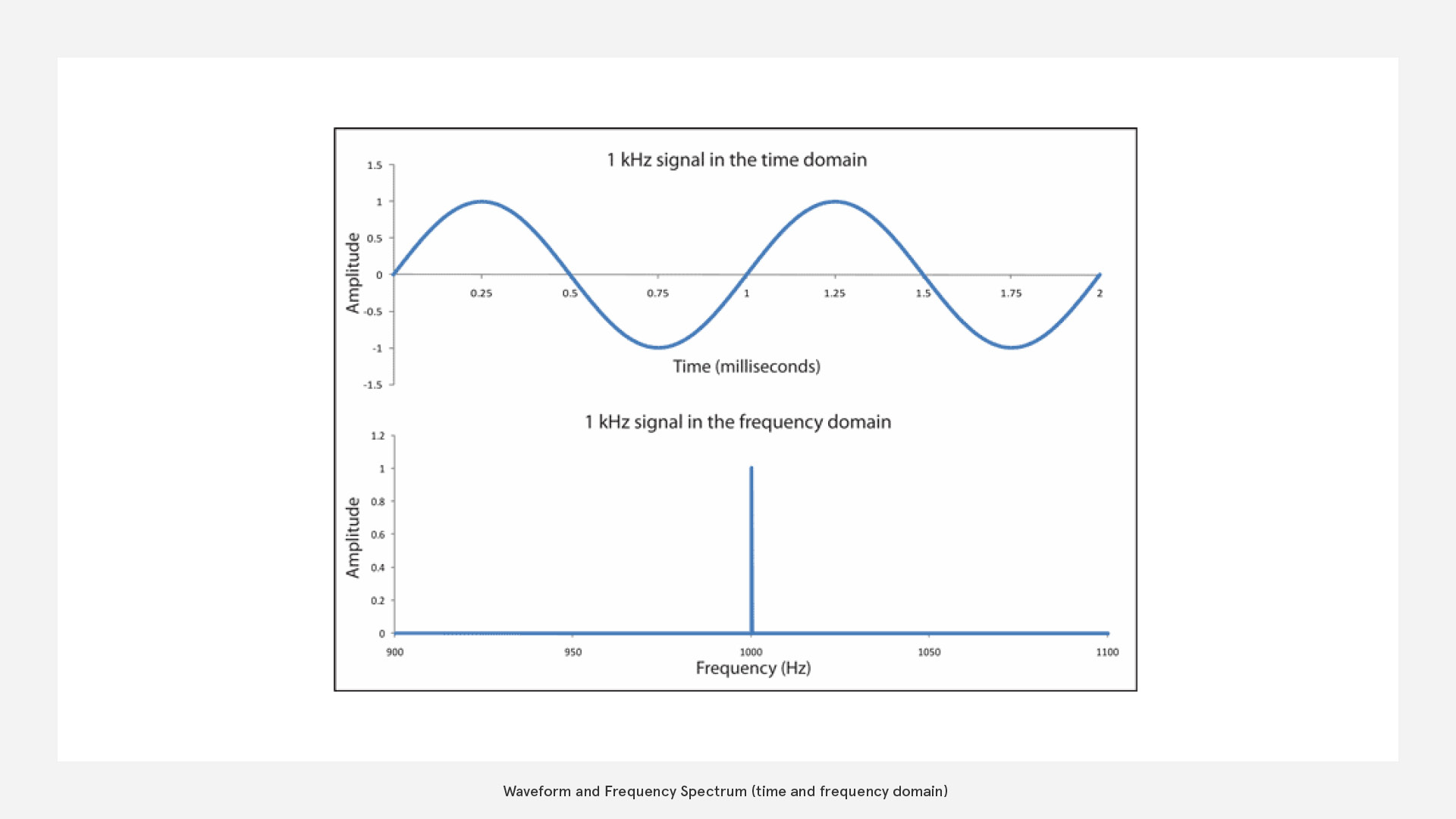
We have already looked at the overall amplitude of a sound signal. Now we want to find the amplitudes per frequency (band). For this we shift from a time to a frequency domain.
FFT
FFT (Fast Fourier Transformation) will provide you with solid data for audio visualisation but needs a bit of an understanding to use it effectively. FFT is a transformation from time domain to frequency domain
How does it work?
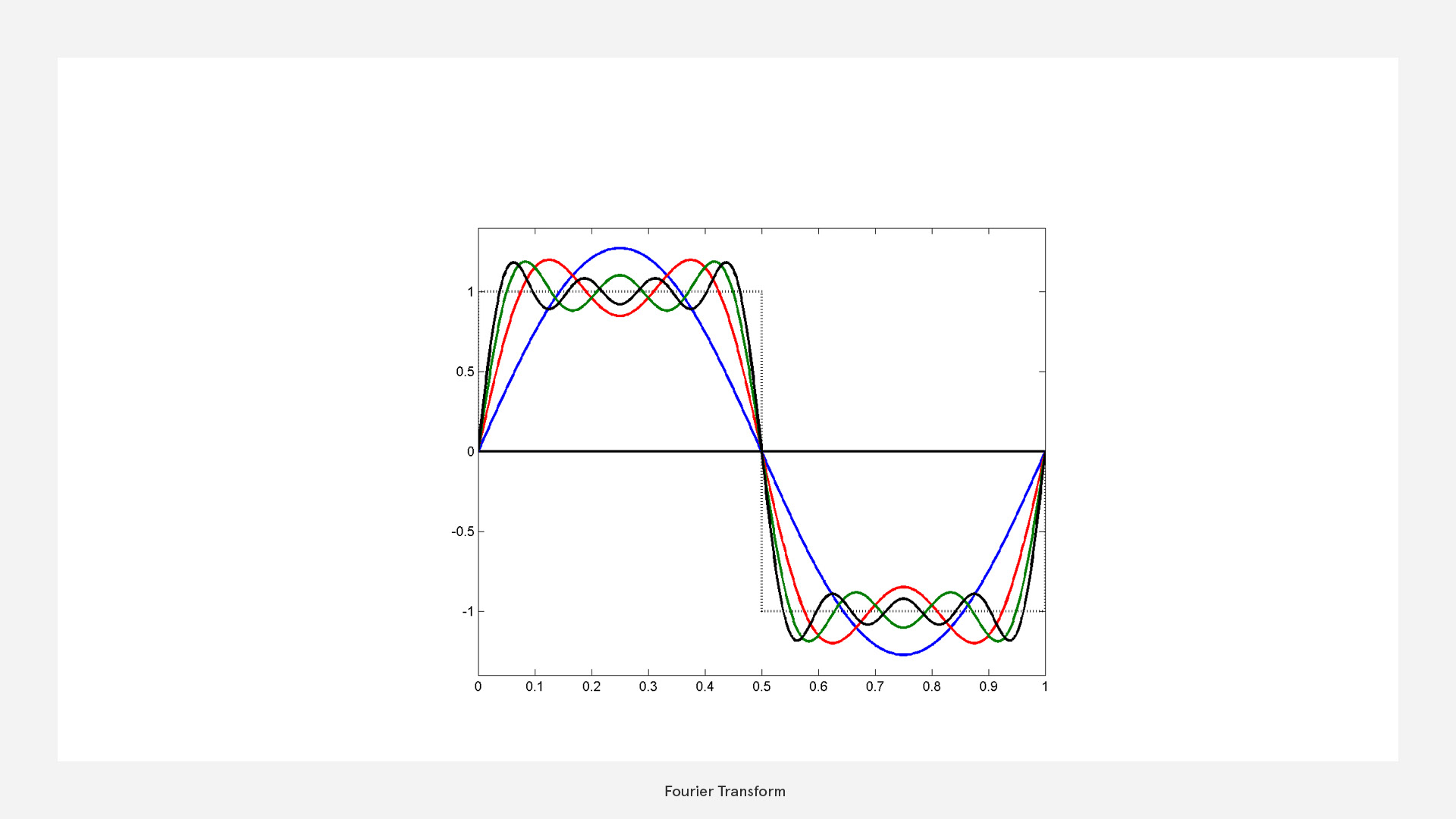
Basically the FFT uses a simple trick: It approximates the waveform with layered sine waves of different frequencies. Through that we find out which frequencies appear in the sound and at what amplitude.
If we try this with a square wave, this would look like this:
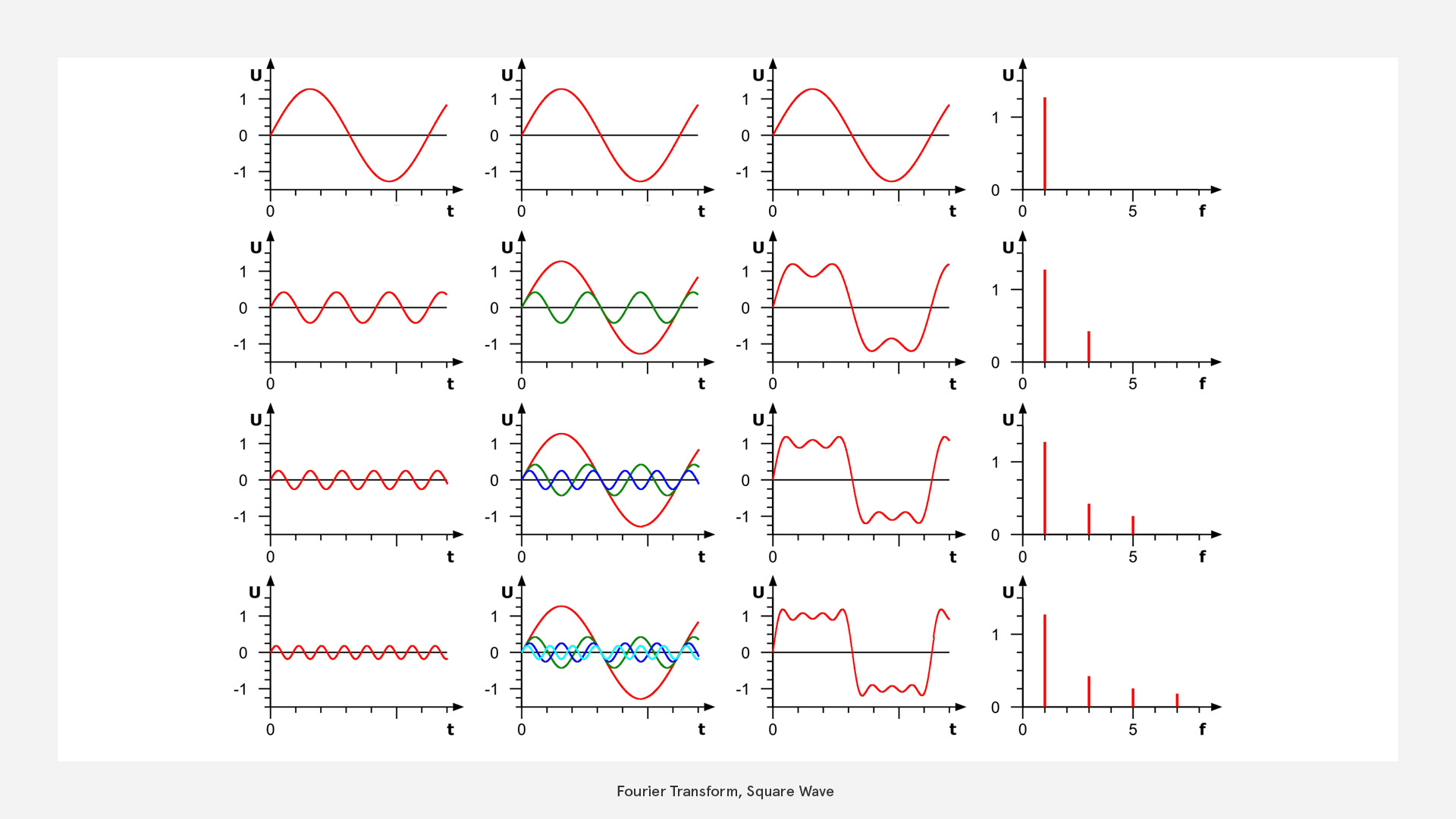 Note that the graphs in the first three columns are in the time domain (x=time) while the last shows the frequency distribution.
How much information can we obtain?
obtainable Information based on Nyquist frequency
As we deal with digital signals, they are sampled at specific sampling rate (a signal resolution) and are therefore limited in their information
Nyquist states that the minimum rate at which a signal can be sampled without introducing errors, is twice the highest frequency present in the signal.
So in reverse this means that the highest frequency we can safely detect is half the sampling rate
eg. in a 44100Hz (CD quality) audio file the highest frequency is 22050 Hz.
How can we interpret the frequency data?
Logarithmic Frequency Perception
Let's think about musical octaves. We know that every octave we experience a note as equal, just higher or lower. By looking at the frequencies we can see that an octave means doubling the frequency. This corresponds to how our hearing is based not on a linear but approximately on a logarithmic scale. (In fact our hearing is almost linear in in low frequencies and logarithmic in high frequencies.)
In a practical sense this means that we can distinguish low frequencies very well, while high frequencies sound all the same to us.
It is important to note, that frequency is not the same as pitch with the only exception of a pure sine wave. While pitch (musical term) describes how high or low a signal sounds, frequency (scientific term) matches the complexity of the actual wavefrom. Think about how you could play the same note (pitch) with a e-guitar and a violin, but the contained frequency structure would be different. They are of course correlated.
So if we combine this knowledge with the Nygquist frequency we start at 22050Hz and for each octave we cut the frequency band in half we get:
| Band | Frequency |
|---|---|
| 1 | 11025 to <22050 Hz |
| 2 | 5512 to <11025 Hz |
| 3 | 2756 to <5512 Hz |
| 4 | 1378 to <2756 Hz |
| 5 | 689 to <1378 Hz |
| 6 | 344 to <689 Hz |
| 7 | 172 to <344 Hz |
| 8 | 86 to <172 Hz |
| 9 | 43 to <86 Hz |
| 10 | 22 to <43 Hz |
| 11 | 11 to <22 Hz |
| 12 | 0 to <11 Hz |
more info here: compartmental on fft
This means that for a audio file with a sampling rate of 44.1kHz we can get data for 12 Octaves. (at least one is already out of our hearing range though)
Equal Loudness Contour
Furthermore, the perception of each frequency's loudness (amplitude) is not linear either - humans perceive low frequencies as less loud ("dull") although they carry high engergy.
 For that reason it is beneficial to take that into account as well by essentially scaling-up the amplitude values from mid to high frequencies.
Usually any pragmatic solution will already help (no need for too much accuracy) - e.g. an envelope that gradually increases scaling from 1...x, between 0...1000Hz
See Equal-loundess contour on Wikipedia
For that reason it is beneficial to take that into account as well by essentially scaling-up the amplitude values from mid to high frequencies.
Usually any pragmatic solution will already help (no need for too much accuracy) - e.g. an envelope that gradually increases scaling from 1...x, between 0...1000Hz
See Equal-loundess contour on Wikipedia
Buffer
For FFT we can not look at an infinetly short slice because there would be no waveform that we could analyse. So we have to decide on a buffer that gives us a large enough slice to extract relevant frequency information. This of course is always a compromise between latency (lag) and frequency accuracy. A longer buffer means being less tightly synced but getting better frequency data.
- use a short buffer to detect onsets
- use a longer buffer for more accurate frequency data
In general FFT with logarithmic averages is much more meaningful if you need a strong correspondence to our perception.
Processing, etc
Again, you are going to find FFT in many frameworks readily available.
- Unity: AudioSource.GetSpectrumData(), in
- Three.js: AudioAnalyser, in
- p5.js: p5.FFT()
- Houdini: volumeFFT SOP, TouchDesigner: Audio Spectrum CHOP ...
In Processing you have minim and processing.audio with their functions. You can quickly check out the basic FFTAnalysis sketch that comes with the processing.audio library. It is very straightforward and for some cases it could already be a good starting point.
But, as we have heard in the introduction, this basic, linear implementation is not very practical, because it doesn't take our perception into account, which is rather logarithmic.
That's why I use the minim library for this exercise, which already provides us with these features. First, let's install the library via the add library from the sketch menu.
FFT Buffer Class
We start by building our own FFTBuffer that contains fewer but more representative values. In that way they are both easier to handle and we have a better approach to pick out individual instruments for things like beat detection, etc.
This is going to be the heart of our analysis and you will benefit from your knowledge of logarithmic scales (remember the table with the octaves)
- I import the libraries into the main sketch (import ddf.minim.; import ddf.minim.analysis.;)
- I create the minim object within the setup() method: Minim minim;
- I create a new tab for my FFTBuffer class and start writing, closely based on the minim examples.
class FFTBuffer
{
  FFT fft;
  public float[] spectrum;
  public int fftSize;

  FFTBuffer(int bufSize, float sampleRate)
  {
    fft=new FFT(bufSize,sampleRate);
    fft.logAverages(22,5);    // 50 bands, 10 octaves
    // >> logAverages(int minBandwidth, int bandsPerOctave)
    // >> see table for comparison: a minimum bandwith of 22Hz means 10 octaves, these get subdived in 5 bands >> 50 values
    // >> fft.logAverages(22,3);  //>> fftSize= 30  // (int minBandwidth, int bandsPerOctave)
    // >> fft.logAverages(11,1); // one band per full octave > fftsize=11:  why not 12? because the first band goes from 0 to <11 (exclusive)
    // >> conflicting: http://code.compartmental.net/minim/fft_method_logaverages.html
    fftSize=fft.avgSize(); //  the length of the averages array
    spectrum=new float[fftSize];
  }

  void update(AudioBuffer mix)
  {
    fft.forward(mix);
    for (int i=0;i<fftSize;i++)
    {
      // spectrum[i]=fft.getAvg(i);                 // >> no damping
      spectrum[i]+=(fft.getAvg(i)-spectrum[i])/4f;  // >> with some damping
    }
  }
}
Photon Class
This is the part that actually draws the visualisation
class Photon
  {
    float x,y,r;
    int bandNr;
    float yOs=2f;
    int col;

    Photon(int _bandNr)
      {
        bandNr=_bandNr;
        y=map(bandNr,
        0 , fftBuffer.fftSize,
        -fftBuffer.fftSize/2 , fftBuffer.fftSize/2) *yOs;
        colorMode(HSB);
        col=color(map(bandNr,0,fftBuffer.fftSize-1,0,255),200,255);

      }

    void draw()
      {fill(col);
       noStroke();
       r=fftBuffer.spectrum[bandNr];
       // r=fftBuffer.env.val[bandNr]*10f; // show env
       pushMatrix();
         translate(0,y);
         rotateX(PI/2);
         //scale(r,r,r);
         ellipse(0,0,r,r);
       popMatrix();

      }
  }
Main
The main class is (as usual) where it all comes together. Note that I've also imported "peasy" - a library for simple 3D camera navigation.
import ddf.minim.*;
import ddf.minim.analysis.*;
import peasy.*;

Minim minim;
AudioPlayer player;
FFTBuffer fftBuffer;
Photon photon[];

//String musicFile="od-stw.mp3";
String musicFile="../data/beats.mp3";
PeasyCam cam;

void setup()
   {size(800,600,P3D);

    minim=new Minim(this);
    cam=new PeasyCam(this,250);
    player=minim.loadFile(musicFile);

    player.play();
    fftBuffer=new FFTBuffer(player.bufferSize(),player.sampleRate());
    println("buffersize=" +player.bufferSize()+"  samplerate="+player.sampleRate()+"  fftSize="+fftBuffer.fftSize);

    photon=new Photon[fftBuffer.fftSize];

    for (int i=0; i<fftBuffer.fftSize;i++)
        {photon[i]=new Photon(i);
        }
   }

void draw()
  {background(0);
  // translate(width/2,height/2);
   fftBuffer.update(player.mix);

 for (int i=0; i<fftBuffer.fftSize;i++)
        {photon[i].draw();
        }

  }
Please, try to reproduce and understand the code in any framework you like
Adjust the visualisation until you are satisfied and until it works well with the audio you picked
Advanced
Windowing
The Fourier Transformation operates on the assumption that the analysed data is periodic (repeating in time) - but in FFT we are actually looking at discreet slices of a waveform. Therefore major glitches (discontinuities) may occure at the edges of theses slices. Windowing is used to lessen this effect. There are several window types - use "Hanning" for most of the cases.